Some would say those are random (stochastic) processes, some would argue that they are chaotic or just purely deterministic (i.e. predictable) but resulting from a succession of factors too complex to understand.
There is however a consensus to describe this uncertainty with laws of probability, the most popular of them being the log-normal law. The log-normal12 law states that the logarithm3 of the considered variable (in our case security prices) is normally distributed. Although this choice is far from being absurd, it has been privileged mainly because it makes all computations much easier.
1. A log-normal (or lognormal) distribution is a continuous probability distribution of a random variable whose logarithm is normally distributed. Thus, if the random variable Xis log-normally distributed, then Y= ln(X)has a normal distribution. Likewise, if Yhas a normal distribution, then the exponential function of Y, X= exp(Y), has a log-normal distribution. A random variable which is log-normally distributed takes only positive real values.
2. The normal distribution is useful because of the central limit theorem. In its most general form, under some conditions (which include finite variance), it states that averages of samples of observations of random variables independently drawn from independent distributions converge in distribution to the normal, that is, they become normally distributed when the number of observations is sufficiently large.
3. The logarithm is the inverse function to exponentiation. That means the logarithm of a given number xis the exponent to which another fixed number, the base b, must be raised, to produce that number x. In the simplest case, the logarithm counts repeated multiplication of the same factor; e.g., since 1000 = 10 . 10 . 10 = 103, the “logarithm to base 10” of 1000 is 3.
4. Parametric statistics is a branch of statistics which assumes that sample data comes from a population that can be adequately modelled by a probability distribution that has a fixed set of parameters.
Without entering into the details of statistics, let us just say that those laws are usually characterised by a set of parameters 4. In the case of log-normal laws, it will be mean and variance.
Thus, in order to accurately describe the possible outcomes of investment in a security, one would need to accomplish the following set of actions:
- Select the appropriate type of probability law for that security,
- Estimate each of the parameters that define the law.
Common practice is to go for the log-normal law and estimate 5 the law’s variance 6 by measuring the security prices’ standard deviation 7 over a certain period of time with a given frequency (daily, weekly…). Estimating the mean is more difficult and is usually not really considered since the aim of the process is to determine risk, which is mainly driven by the probability law’s variance.
5. Estimation is the process of finding an approximation derived from the best information available.
6. The risk of a portfolio is usually represented by various terms (volatility, Value-at-Risk…) that all relate in some way to the variance of the probability law, which can be seen as the square of its standard deviation.
7. The standard deviation is a measure that is used to quantify the amount of variation or dispersion of a set of data values. A low standard deviation indicates that the data points tend to be close to the mean of the set, while a high standard deviation indicates that the data points are spread out over a wider range of values.
Two remarks need to be made at this stage:
- Estimation always includes some part of error,
- Security prices usually don’t strictly follow a log-normal law (or any other common law).
Estimation errors arise because the sample of prices is just one set of observations of the probability law. It’s like tossing a coin 5 times: there is no way you will get a 50-50 split of outcomes, and there is even a small probability that you will get 5 heads in a row. Estimating probabilities from this sample would result in a 100% probability of getting heads and 0% risk…
There are two ways to tackle this problem. The first is to try to reduce the errors as much as possible by using more complex probability laws and estimation process. The second is to try to reduce as much as possible the impact of the sampling errors on the estimation process and their consequences on the decision making process based on those estimations.
The second way has led to the development of a branch of statistics (robust statistics) and the development of statistics that do not require hypotheses on parametric laws.
One simple example is Spearman’s ranks correlation. It is used as a substitute to usual (linear) correlations to detect a relationship between two sets of data even if the relationship is not linear.
Reference Portfolio (RPo) follows this second way, using at every steps tools that spare us the challenges of choice of laws and estimation of parameters as much as possible.
We will illustrate in the following sections the concrete benefits of this approach.
2. Estimation errors and asset allocation
A first question is to determine the type of error one might make in estimating the risk characteristics of common asset classes.
To get a rough estimate of the magnitude of this problem, we have selected four asset classes:
- Euro Equities,
- World Equities,
- Euro Bonds,
- World Bonds.
Each asset class is represented by an index, with data ranging from 31/10/2005 to 5/10/2018. We have measured the volatilities (standard deviations) and correlations of those 4 asset classes with 4 different methods:
- Daily on the first half of the data (2005-2012)
- Monthly on the first half
- Daily on the first half (2012-2018)
- Daily on the second half
Each of those measures is an acceptable estimate of the “real” risk characteristics of those asset classes. However, we will see that they yield quite different results.
The results of those measures yield the following results:

CORRELATIONS
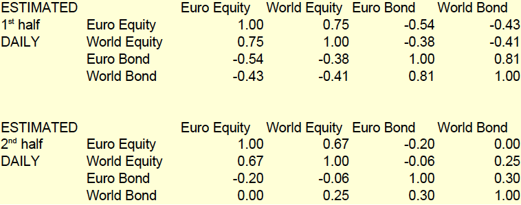
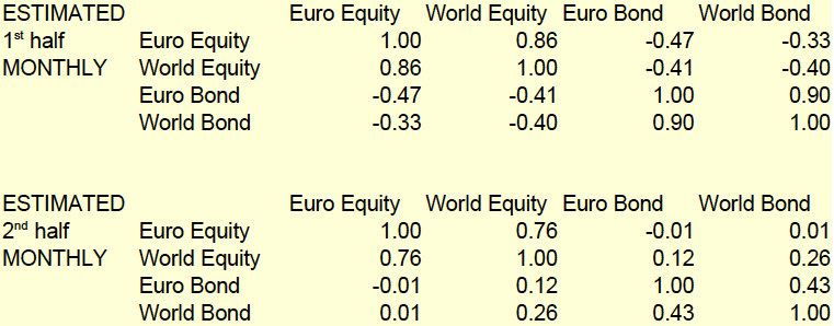
On this example, the range of error goes from 1.3% (Euro Bond) to 11.3% (Euro Equity). The largest gap in terms of correlations is 0.53 (Euro equity vs Euro Bond).
We will use those figures to determine a likely scenario demonstrating the advantages of Reference Portfolio (RPo).
3. Portfolio construction and estimation errors
In order to assess the impact of estimation errors on portfolio construction, we will now assume that we “know” the real risk and correlation figures, and we will compare portfolios resulting from “real” figures to those resulting from a set of purposefully error-stained figures (called Estimated), for the sake of illustration.

The average error in volatility estimation is -17% of real risk.
CORRELATIONS
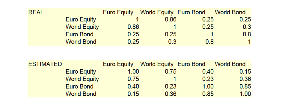
In order to get rid of the problem of returns estimation and risk aversion, we will just build the minimum risk portfolio from those 4 asset classes.
The real and estimated portfolios are constructed by minimising the risk of the portfolio using respectively the real and estimated risk and correlation matrices. It is thus the true minimum risk portfolio, and by definition other “minimum risk” portfolios, being based on erroneous estimated figures, will be riskier due to error estimations.
Reference Portfolio (RPo) is a dual risk system using a reference allocation as a starting point. In this example, we will use an equally weighted portfolio with 25% in each asset class and deform it by reducing the equity weight and increasing the bond weight until we reach the minimum risk according to the estimated risk and correlation matrices.
The results are as follows:
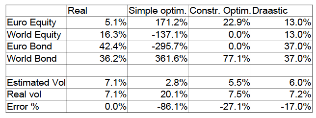
For the Real portfolio, estimated volatility=real volatility by definition. For the unconstrained portfolio (i.e. long and short positions allowed), the estimated volatility is 2.8% but the real volatility is 20.1%, 7 times higher. Even the constrained (weights>=0) minimum risk portfolio almost doubles the average estimation error with an estimate of 5.5% vs a real volatility of
7.5%, while Reference Portfolio (RPo) portfolio’ error on volatility is in line with the average estimation error (-17% in both cases) with an estimate of 6.0% vs a real volatility of 7.2%.
4. What is good diversification?
The sample data we have studied shows that seeking diversification based only on historical prices’ correlations and volatilities can be a tricky choice.
Since past correlations are not fully reliable, we have decided to turn to “second order” criteria for diversification in Reference Portfolio (RPo). Those are:
- Naive diversification (i.e. equal weights)
- Market cap weights
- Domestic preference
First and foremost, naive diversification is what protects the investor in the case of one asset (or asset class) experiencing a sharp drop. It is especially useful when this possibility is not reflected in past prices, i.e. when the asset class was highly correlated in the past with some other asset class.
Let us take the example of Greece Government Bonds in the late 2000s. Being denominated in Euro, they were seen as highly correlated with German or French bonds. Since their yield was slightly higher than their French or German counterparts, it would have been quite possible to have a portfolio highly concentrated in Greek bonds. But as the probability of a credit default from Greece grew stronger, the Greek bonds plunged much faster than other Euro-denominated bonds during the crisis. In such a situation, naive diversification would have limited the exposure to Greek bonds.
Market capitalisations are another way to diversify risk, as they represent a form of market consensus on risk- and return-adjusted correlations.
Domestic preference is the most subjective of the 3 criteria. It is justified by the fact that domestic assets often have some form of tax incentive for investors. Another justification is that domestic markets follow more closely the domestic economy, which is an implicit benchmark for some investors. And last, domestic assets are not subject to foreign exchange risk, which spares the cost of hedging this risk, even if that cost is usually rather low.
Those criteria are used to build a reference portfolio (Rpo) as to compare approaches.
5. Impact on performance
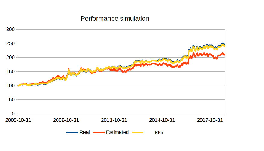
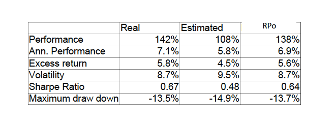
The estimated (constrained optimisation) portfolio exhibits a higher risk and lower return than Reference Portfolio (RPo) portfolio on our sample data. Note that estimated portfolio may also have higher returns if the assets for which risk is underestimated happen to outperform other assets, but the actual risk will always be higher than the target (estimated) risk.
The impact of estimation errors is even bigger if we use those portfolios as the risky portfolio in a portfolio insurance (CPPI) process. Since the optimal multiplier depends on the estimated risk of the risky portfolio, the underestimation of risk will result in a multiplier higher than it
should be, and lesser performance because of trading costs that will be higher than the gain in performance.
We will now implement a strategy protecting 80% of the highest portfolio value at any time, using the 3 portfolios we have generated as the risky asset of the CPPI strategy.
We choose a protection of highest portfolio value in order to keep an active protection strategy during the whole back testing period. Otherwise, as the markets were globally bullish, the only active period would be the first few years.
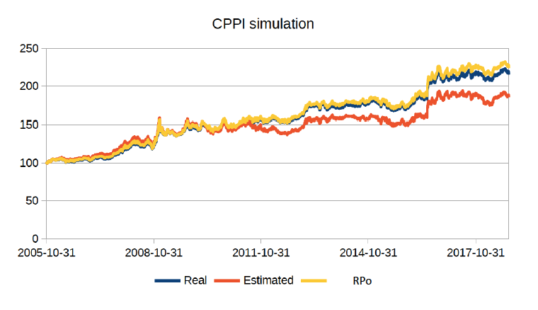

We see that, due to the underestimation of risk, the CPPI strategy based on the estimated (constrained optimised) portfolio yields 21% of the initial performance, while the Reference Portfolio (RPo)-based CPPI portfolio yields only 10% of its initial performance.
6. Choosing the right probability law (or not choosing)
So far, we have used asset classes that do not stray too far from the log normal law, so the use of correlation matrices was quite acceptable. But what if we add asset classes that are far from following such probability laws?
There is abundant literature documenting this phenomenon. Let us first mention Benoit Mandelbrot, who started his fractal theory because he observed that commodity prices were often experiencing price changes that, according to log normal-laws, should happen only once per century, if not less. Nassim Taleb also built strategies like the Black Swan on the same sort of observations.
Let us just say that those phenomenon happen in real life, especially in alternative investments. In that case, using a log-normal probability law is quite inappropriate, but which law should we choose? Levy, truncated Levy, exponential? And there is still the need to estimate the parameters.
Here Reference Portfolio (RPo) follows another way, using historical Value-at-Risk.
To illustrate the problem, we have selected the HFRX Convertible Arbitrage index, which is a good example of how some prices in finance can be extremely un-log-normal.
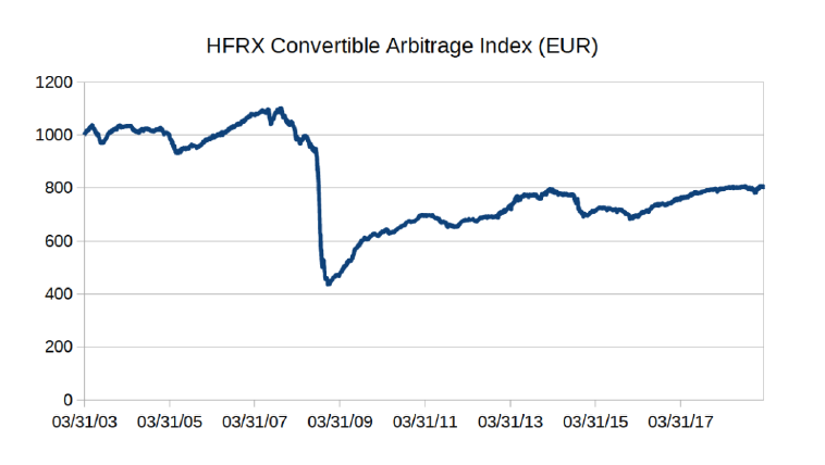
If we consider that this series of prices is representative of the risk characteristics of the index, what is the best way to compute extreme risk, namely the 99% 1 year Value-at-Risk.
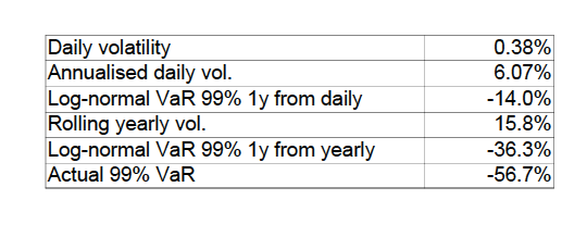
We can see that Value-at-Risk estimated from a simple log-normal approach are very far from the actual historical VaR. And volatility-based figures are clearly lacking consistency between daily (-14%) and yearly (-36.3%) estimations.
Choosing the wrong law of probability can lead to wrong estimations and huge mistakes on risk estimation, while historical Value-at-Risk, by avoiding the necessity of choosing a law, will in any case give an acceptable estimate of the actual risk.
The problem gets even worse when it comes to estimated aggregated risk, i.e. the risk of a portfolio containing Convertible Arbitrage plus other asset classes.
The use of linear correlation matrices is justified in the case of log-normal variations only but can be tricky when some of the assets have risk characteristics that differ significantly from a log-normal law.
7. Beyond historical value-at-Risk
The choice of historical Value-at-Risk as the standard risk measure in Reference Portfolio (RPo) is justified not only for theoretical reasons, but also for practical ones. In this context, it is very easy to add an asset class as long as we have some daily historical data available.
However, some asset classes, like Private Equity, do not offer this kind of long daily history. This is why Reference Portfolio (RPo) is designed to integrate parametric risk measures for asset classes that cannot fit in the historical VaR framework.
8. About risk premia
The most important factor in future performance is the expected return. Unfortunately, it is also the hardest to forecast. Averaging past realised returns will give a very unstable estimation, with a high dependency to the estimation period.
For interest rate based products, the average yield to maturity can be considered as the market consensus for future returns.
When it comes to equities and hedge funds, there is no such market consensus available. The commonly accepted way of estimating future returns for those asset classes is to consider the existence of a risk premium. This means that investors must receive an incentive to buy
higher risk assets rather than low risk bonds. This incentive is the risk premium, the extra return over the bond yield that compensates the extra risk. Several studies show that this risk premium is rather stable over the long run, around 4% per annum for equities.
For alternative assets, as there are many strategies that are not necessarily consistent over time, we have chosen a Sharpe ratio based approach. In order to keep a relative consistency between asset classes, the expected return of alternative assets is the one that leads to a Sharpe ratio equal to the average Sharpe ratios of the other asset classes.


